Single-Pass vs Lift-Mode KPFM: How HD-KFM Works

Key takeaways

Lift-mode (two-pass) KPFM measures the potential 10–100 nm above the surface on a second pass; single-pass HD-KFM measures it in the same pass, 0.1–0.5 nm from the surface.
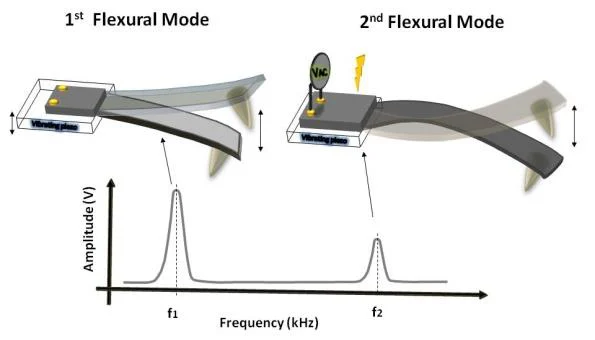
HD-KFM excites the first eigenmode mechanically for the topography and the second eigenmode electrically for the potential, so the signal is amplified by the Q factor of that mode.
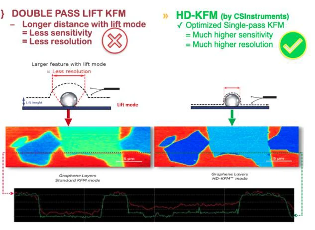
Closer measurement means higher sensitivity and resolution: on the same graphene flake, layer contrast is sharper in HD-KFM than in lift mode (Figure 3).
HD-KFM III adds the capacitance gradient (dC/dz) and Electric Field Cancelling (EFC) for combined KPFM–MFM measurements.

CSInstruments · Updated October 2026

Principle

What KPFM measures

Kelvin probe force microscopy (KPFM, also called KFM) measures the contact potential difference V_CPD between a conductive tip and the sample at each pixel. V_CPD follows the difference of work functions between tip and sample, so a KPFM map is a map of local surface potential and work function — of doping, charge, band bending or layer number, depending on the sample.

An AC voltage applied between tip and sample creates an oscillating electrostatic force; a feedback loop adjusts a DC voltage until the component of that force at the excitation frequency vanishes. The DC voltage that does this is the surface potential. How and where that force is detected is what distinguishes lift-mode from single-pass KPFM.

Two passes

Lift-mode (double-pass) KPFM

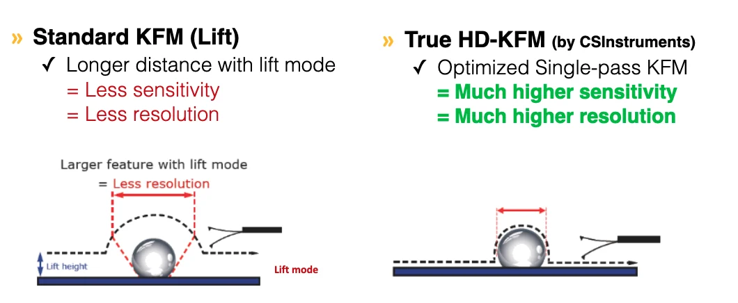
Most KPFM set-ups scan each line twice. The first pass records the topography; on the second, the tip retraces the same profile lifted above the surface — typically 10 to 100 nm — and the potential is measured there.

Resolution and sensitivity — the electrostatic force falls off with distance and the tip interacts with a larger area, so small features are blurred (Figure 1).
Time — every line is scanned twice.
Crosstalk — topography can leak into the potential image.

Figure 1. Lift-mode KFM (left) measures the potential at the lift height, so a feature appears larger and with less contrast; single-pass HD-KFM (right) measures it in the same pass, close to the surface.

Single pass

How HD-KFM works

HD-KFM (High-Definition Kelvin Force Microscopy) uses multifrequency excitation. The first flexural eigenmode of the cantilever is excited mechanically and tracks the topography; the second flexural eigenmode is excited electrically and tracks the surface potential, with two lock-ins and two independent feedback loops. The software finds the second-eigenmode frequency (around 350–400 kHz) and tunes it automatically.

Signal amplified by the Q factor of the second eigenmode, so a smaller AC voltage gives an acceptable signal-to-noise ratio.
Stability from the stiffer effective spring constant of the second eigenmode.
Close to the surface — typical minimum tip–sample distance of 0.1–0.5 nm, against 10–100 nm in double-pass KFM.

Figure 2. Multifrequency excitation in HD-KFM: the first flexural mode (f1) for topography, the second flexural mode (f2) for the surface potential.

Results

Lift mode and HD-KFM on the same sample

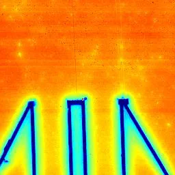
Figure 3. Graphene layers, same area, 5 µm scale bar: standard lift-mode KFM (left) and HD-KFM (right), with the line profiles of both (red: standard KFM, green: HD-KFM). Layer boundaries are sharper and the levels flatter in HD-KFM.

A simple check of any KPFM set-up is a structure whose potential is set externally. In Figure 4, three linear electrodes on silicon are biased at 1 V: HD-KFM shows a homogeneous potential on the electrodes and the lateral diffusion of the potential around them.

Figure 4. HD-KFM image (10 µm) of three linear electrodes on a silicon surface biased at 1 V: homogeneous potential on the electrodes (dark blue) and lateral diffusion around them (cyan).

HD-KFM III

More than surface potential

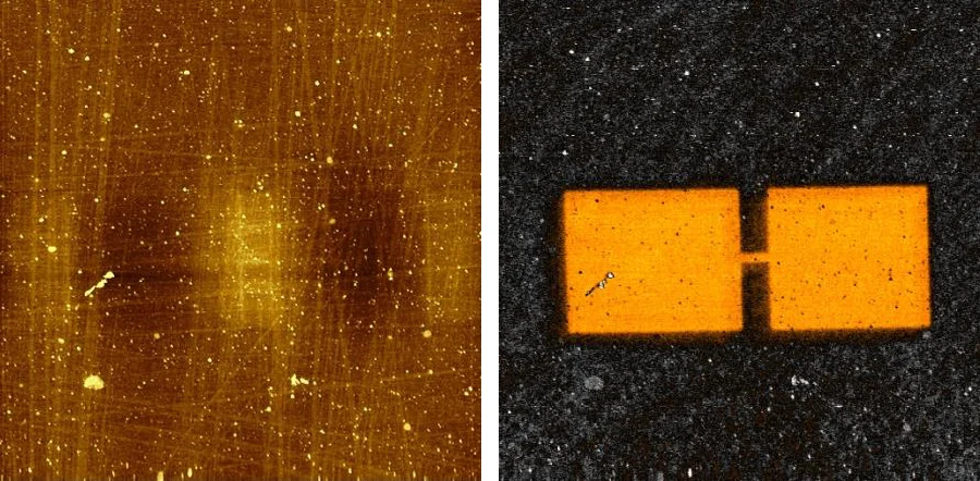
Capacitance gradient (dC/dz). The electrostatic force also has a component at twice the excitation frequency, proportional to dC/dz. Tuning a lock-in to it maps the local dielectric properties at the same time as the potential (Figure 5).

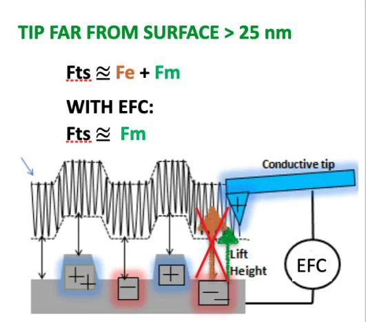
Figure 5. Metallic structure embedded in epoxy: topography (left) and dC/dz (right). The structure barely shows in the topography but is clear in the capacitance gradient.

Electric Field Cancelling (EFC). Far from the surface, as in MFM, the tip feels both magnetic and electrostatic forces. EFC compensates the electrostatic part, so that MFM shows magnetic contrast only and HD-KFM and MFM can be combined (Figure 6).

Figure 6. EFC principle: with the tip more than 25 nm from the surface, the total force is electrostatic plus magnetic; with EFC it is the magnetic force only.

Sub-surface detection. Electrostatic interactions are long-range, so HD-KFM also reveals charges and structures below the surface, such as carbon nanotubes in a polymer matrix.

Summary

Lift-mode KPFM vs single-pass HD-KFM

	Lift-mode (double-pass) KPFM	Single-pass HD-KFM
Passes per line	2 — topography, then potential	1 — topography and potential together
Tip–sample distance for the potential	typically 10–100 nm (lift height)	0.1–0.5 nm
Electrical detection	at the lift height	second eigenmode, amplified by its Q factor
Topography crosstalk	possible from the retrace	no retrace
Extra channels	—	dC/dz; EFC for combination with MFM

HD-KFM™ III runs on the Nano-Observer II, HD-KFM™ I on the Nano-Observer One Plus, and existing MultiMode, Dimension and Agilent AFMs gain it with the Galaxy Dual Controller.

KPFM in practice

HD-KFM™ IIIKelvin probe force microscopy (KPFM)KPFM on perovskite solar cellsHD-KFM on 2D materialsHD-KFM and ResiScope on semiconductor devices

FAQ

Frequently Asked Questions

What is single-pass KPFM?

Single-pass Kelvin probe force microscopy measures the topography and the surface potential during the same scan line, instead of scanning each line twice. In HD-KFM, the first flexural mode of the cantilever follows the topography while the second eigenmode is excited electrically to measure the potential.

What is lift-mode (two-pass) KPFM?

In lift mode, each line is scanned first to record the topography, then a second time with the tip lifted above the surface, typically 10 to 100 nm, to measure the surface potential.

Is single-pass KPFM better than lift-mode KPFM?

Measuring closer to the surface gives higher sensitivity and lateral resolution: HD-KFM works with a tip–sample distance of 0.1 to 0.5 nm, against 10 to 100 nm for double-pass KFM. It also avoids the second pass, which doubles the acquisition time and can let topography leak into the potential image.

Why does HD-KFM use the second eigenmode of the cantilever?

The electrical signal is amplified by the Q factor of the second eigenmode, which allows a smaller AC voltage for the same signal-to-noise ratio, and the stiffer effective spring constant of that mode adds stability. The software finds and tunes the excitation frequency automatically.

Can KPFM detect structures below the surface?

Yes. Because electrostatic interactions are long-range, HD-KFM can reveal charges and structures buried under the surface, such as carbon nanotubes embedded in a polymer.

Can KPFM be combined with MFM?

Yes. HD-KFM III and MFM can be measured together, and the Electric Field Cancelling (EFC) option compensates the electrostatic force so that the MFM image shows magnetic contrast only.

How is a KPFM measurement checked or calibrated?

On a sample with a known potential — for example electrodes biased at a set voltage — and, for work-function values, by calibrating the tip on a reference such as freshly cleaved HOPG.

Questions about KPFM or HD-KFM™?

Ask the application scientists behind our AFMs and modes — about your samples, probes, set-up or which mode fits your measurement. We answer every message personally.